I’m not going to present SQL. I’ve written a fair amount of SQL, queries of many shapes and sizes. I’ve done a lot of mistakes and debugged many performance issues in SQL. Thus, overall, I’m decently competent in SQL and claim to have some credibility in assessing how SQL is taught in tutorials. If you type “left join SQL” into Google Search, you’ll likely be presented with pictures that resemble Venn diagrams.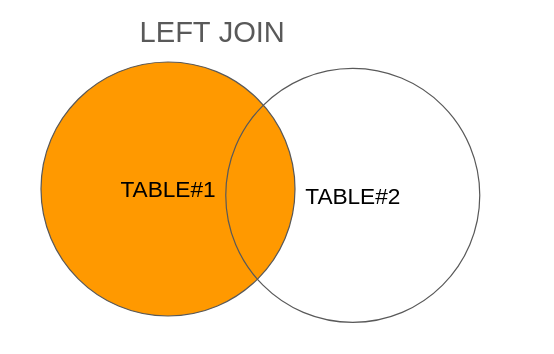

I hope you’ll never have to resort to such subpar tutorials again, and I feel sorry for you if you had to rely on them in the past. These diagrams are fundamentally flawed and I’d even go so far as to call them lazy. They’re so lazy that I took the 10 seconds it would have taken to create a proper one and spent that time crafting an example to illustrate my point without having to give credit to any tutorial website.

The above picture is incorrect. The above picture is a Venn diagram illustrating two intersecting sets, with one of them colored. However, that’s not what an SQL join is about. Let me elaborate.

Let’s start from the basics. What is a SQL table? answer: a collection of records, you can consider them as Sets or as Bags in mathematical formalism. I prefer to consider them as Sets with some surrogate “positional-number” key so that no two records in a same table are “equal”.

What is a SQL join? Answer: an operation that performs the Cartesian product of two tables. Hence, it’s a SetA -> SetB -> SetC function, where SetC is defined as some bastardized (SetA x SetB). That is, a join cannot be illustrated with a Venn diagram: the three tables - SetA, SetB, and SetC - are of entirely different nature, whereas a Venn diagram makes sense for sets of the same nature. The picture of the Venn diagram would lead you to believe that somehow we construct the left join from SetA combined with some part of SetB. I could somewhat make sense of Venn diagrams for INNER joins, but in general, the illustration is misleading and completely remote from reality when discussing FULL joins.

Let’s build a more engaging illustration of what joins are, with some non-lazy pictures. Then, for those willing to venture out of their comfort zone, I’ll make an optional detour: grasping what an SQL engine does by treating SQL engines as predicate machines.

so what is a join anyway?

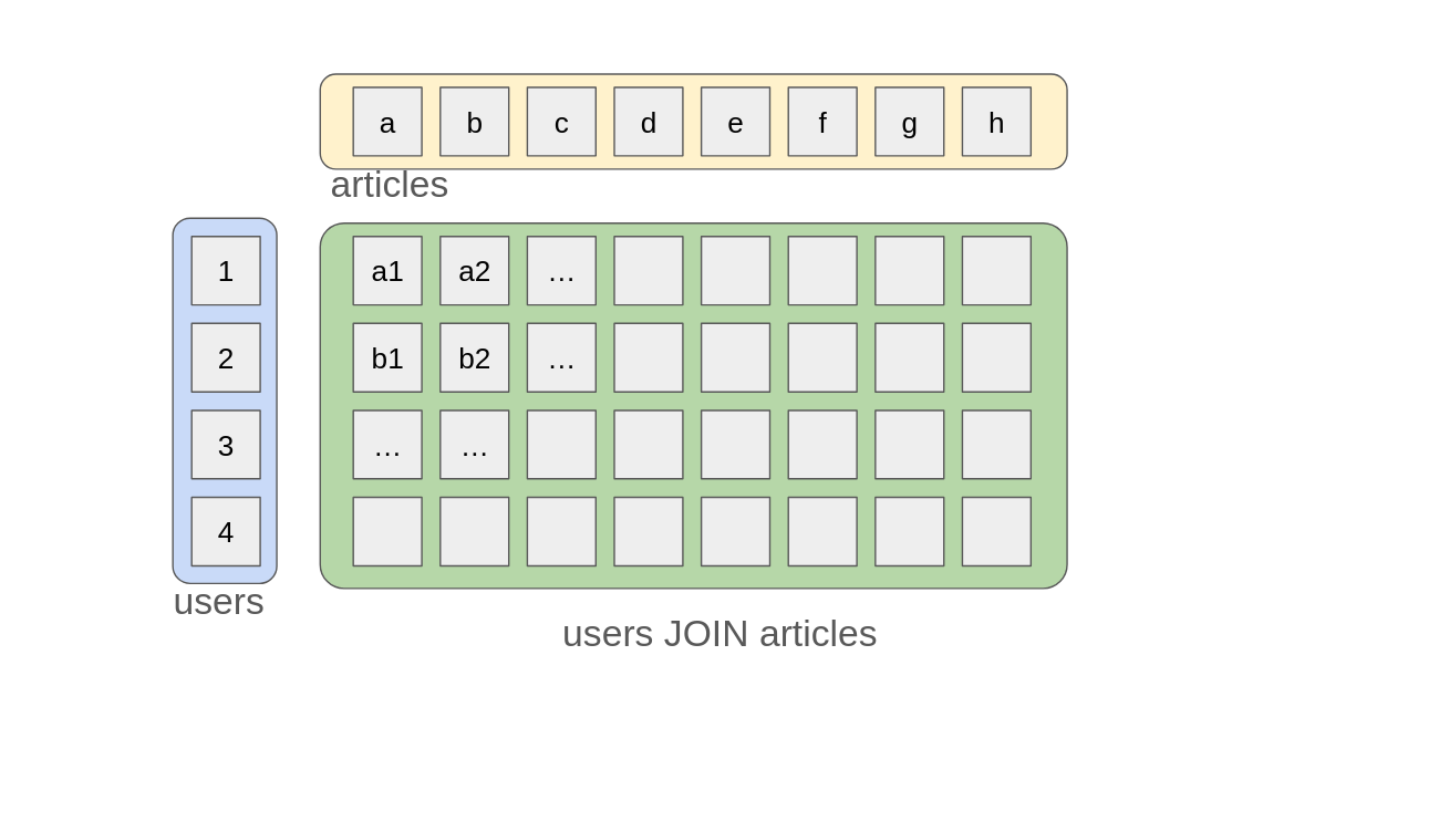
Without further ado, let’s consider the articles table and the users table. We can represent these sets as two aligned vertical lines and a horizontal line, respectively. To join them, we would simply draw a rectangle that encompasses all possible combinations of articles and users.

Here is the rewritten paragraph:

Voilà, you now have a joined users and articles table. In SQL, you’re forced to specify an ON clause. Therefore, this ON must convey some meaning. I believe the ON clause should be optional (in the context of teaching). You can simulate it by doing SELECT * FROM users INNER JOIN articles ON TRUE, it will work, and the resulting set will contain m*n rows if you have m users and n articles.

Most often, the ON clause exists because we want to capture specific relationships, such as which article has been written by which user. This allows us to avoid assuming all articles have been authored by all users. However, this “authorship” relationship between articles and users is a specialized case. We can imagine more complex queries that search for users who have liked certain articles, or articles that cite specific users, or even more intricate relationships such as articles citing users at least three times. The problem SQL beginners encounter here is that tutorials, frameworks, and ORMs tend to conflate different concepts: (i) crafting properly designed SQL queries to enforce business rules, and (ii) schema-modeling intended to encode fundamental ownership relationships.

Let’s illustrate with an example of a join: colouring all items that match our ON predicate.

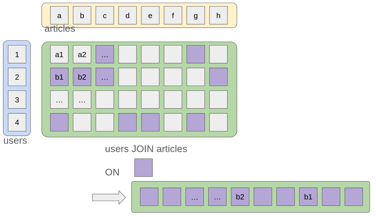
I’ve also shown a flattened version of the joined data because SQL is “uniform” in the sense that the result set is yet another table that could be joined again. Such a picture also illustrates that the process of flattening imposes on picking some ordering (e.g., preferring top to bottom or left to right), hence the SQL engine can take the simplest unless you constrain the query with the ordering you prefer. This reasoning lets us understand that “it makes sense” for an extra filter like a “where” clause to occur before an “order” clause. Indeed, the flattening is made simpler by having fewer items first, conversely, the flattening would make filtering more difficult by removing optimization opportunities like SQL indexes.

What’s left is illustrating what LEFT and INNER join are and how they differ.

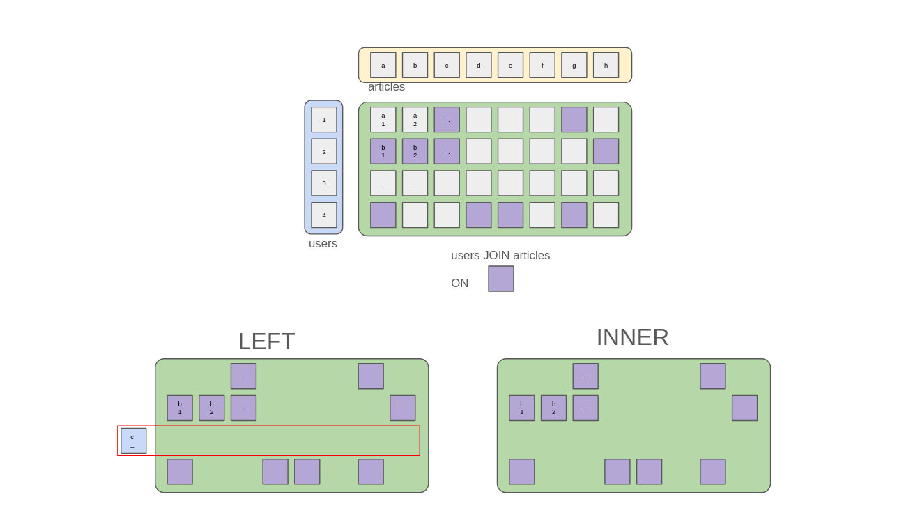
In the above picture, I’ve shown what an INNER join and what LEFT joins are. The INNER join only returns the items that were coloured inside the table. Whereas the LEFT join also considers that if a “user row” has no matching “user x article” square in the joined set, then we still keep a record for the item. Since we cannot attach article information to the “user x article” square, then our result set is somewhat heterogeneous and contains squares of distinct natures (henceforth, my rant about Venn diagrams). You’ll likely have guessed that a RIGHT join is the same procedure as the LEFT join but with adding square items for “article columns” without “user x article”. The FULL join is when we add both (henceforth yielding three types of tiles).

To conclude this section, I hope you’ll find the picture and explanation clear enough. With a bit more pixels and a bit more words than the usual “left join” figure, we can give a better recount of what joins are, how a LEFT or INNER join differs. If you’re set to read or write a lot of SQL, it’s better to build a mental model that serves well when writing and reading SQL queries. To go beyond and be able to grasp what makes a particular query costly or not efficient.

a roundabout way to grasp what SQL tables and joins are about

Furthermore, to fully grasp what a SQL join is, it may be helpful to represent a SQL table as sets rather than concrete collections of rows, but rather as predicates from a given type defined by the table’s “columns”. (I must admit that I find the terms “column” and “row” somewhat antiquated.) Say a table has two columns: age and username. Provided an Oracle function answering questions like: does the record exist with age=32 and username="bob"? Such an Oracle function would have type Age -> Name -> Boolean. Then we can enumerate all possible combinations of Age and Name to fully “reconstruct” the table. We could also “scan” the table and tell whether we found such a record, hence implementing an Oracle function. Therefore, the table data on disk and the predicate function are essentially equivalent: although a predicate could encode an infinite number of values, the table data on disk is finite and limited by storage constraints.

Using this formalism, we can write the types of our sets interpreted as oracles SetA = A -> Boolean, SetB = B -> Boolean, and hence our joined table SetC = C -> Boolean = (A x B) -> Boolean. Substituting these equivalences inside our join function SetA -> SetB -> SetC, we get that join is (A -> Boolean) -> (B -> Boolean) -> ((A x B) -> Boolean). In plain English, we have to grasp that a join is a way to produce an oracle function from two oracle functions. We don’t need any limitations about having items on disk; we don’t need to discuss foreign keys. Now the ON part that SQL forces onto you is a way to further restrict the ((A x B) -> Boolean) predicate. The LEFT, INNER, and OUTER qualifiers modify the type of the resulting set. Instead of answering on ((A x B) -> Boolean), the modified joins may start answering on ((A x B*) -> Boolean) with B* being “a B or a NULL”.

The advantage of this formalism is that it is especially powerful. Predicates can be arbitrarily complex. The problem with this formalism is that it is incredibly inefficient. Just imagine having to enumerate all the possible int and varchar(32) just to know if Bob is in the database! The most obvious optimization a database can do is store and keep only the data supposed to exist in the table rather than storing on disk all combinations of the data rows that don’t exist (note to self: it could be an interesting artistic project to create such an anti-database). As a result, databases perform clever and advanced analyses to determine if they can expedite building a result set. Such a query analysis will scrutinize whether the ON restriction uses predicates on columns that are properly indexed (e.g., an index is sorted so we can perform some dichotomic lookups). More advanced analyses will check whether the predicates can be decomposed into simpler ones (e.g., a conjunction of multiple restrictions, some of which can be accelerated with indexing) or if ON and WHERE restrictions are redundant with each other.

Note that I’m not advocating in favor of teaching SQL tables and joins in terms for general users. However for backend developers who have some mileage already and feel intimidated when reaching for SQL, this formalism can be useful to map-down the complexity of SQL into a more familiar mental model. Finally, this formalism helps in bringing tricks from #constraints programming and #logic programming into your queries to make them more efficient SQL queries (things like self joins of a table on a lexicographical order).

conclusion

We should reject Venn diagrams as an illustration of SQL joins. We can do much better; I hope this article, with a non-lazy illustration and some hand-waved explanations, will prove my point. That’s all.